Before we start using R, we will need working installation of R on our computer. In this blog we will install R (for Windows and Mac OS) and have a quick tour of R environment.
R Installation
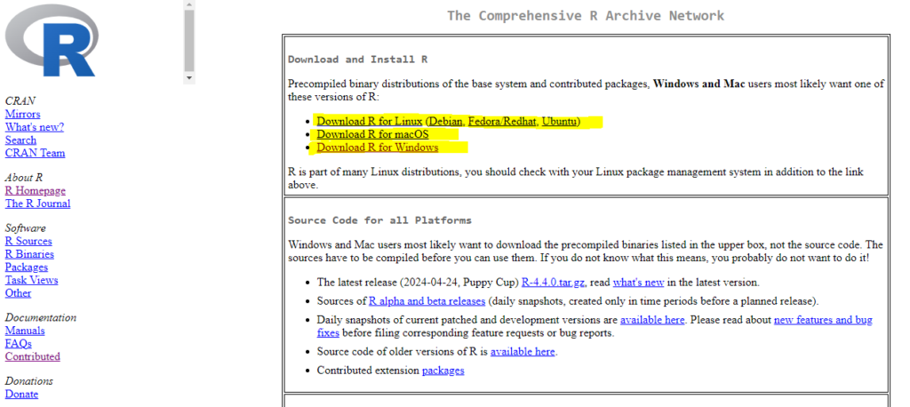
To install R, visit Comprehensive R Archive Network (CRAN) website. CRAN is a network of servers around the world on which R binary files are hosted. Here R packages and documents can be downloaded.
You will be directed to the CRAN home page. On top of the page you will find a box with three links that refer to different download options depending on your operating system. Choose the one that applies to your machine.
Windows User
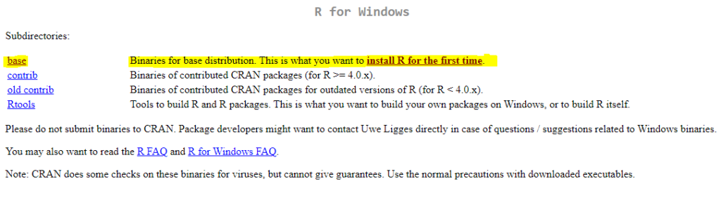
For Window users, select Download R for Windows link and then on base link and finally the download link Download R-4.3.3 for Windows. Please note, R-4.3.3 is latest R version number.
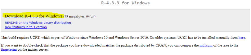
when you click on Download R-4.3.3 for Windows link, this will begin the download of .exe installation file. When download is completed, double click on the R executable file, and follow the on-screen instructions. You can run executable file with all default options. Full installation instructions can be found at CRAN website under R for Windows FAQ.
Mac Users
For Mac users, select Download R for macOS link . The binary can be downloaded by clicking R-4.3.3-arm64.pkg link.
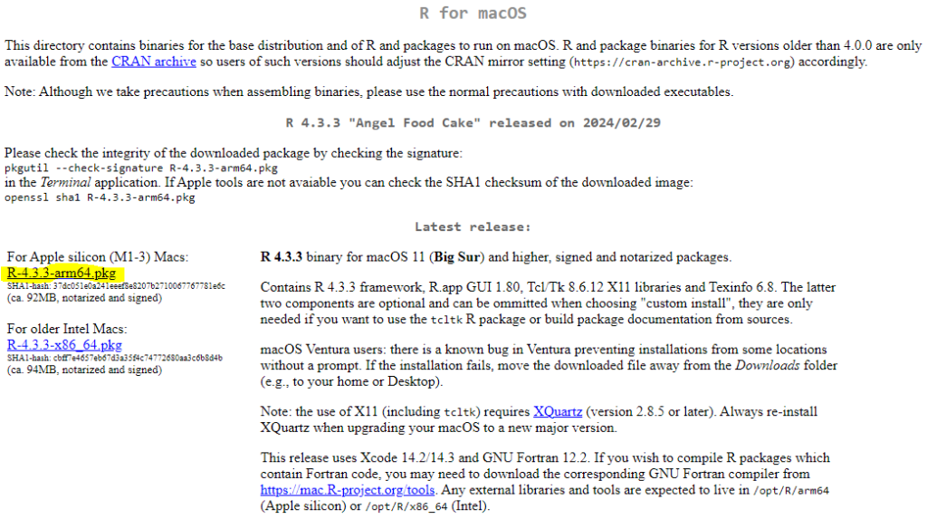
When you click on R-4.3.3-arm64.pkg link, this will begin the download of .exe installation file. When download is completed, double click on the R executable file, and follow the on-screen instructions. You can run executable file with all default options. Full installation instructions can be found at CRAN website under R for Mac OS X FAQ.
R Interface
Once download is complete, double click on R icon to open the R console. In the R console, you will find the latest R version number and some commentary in R project.
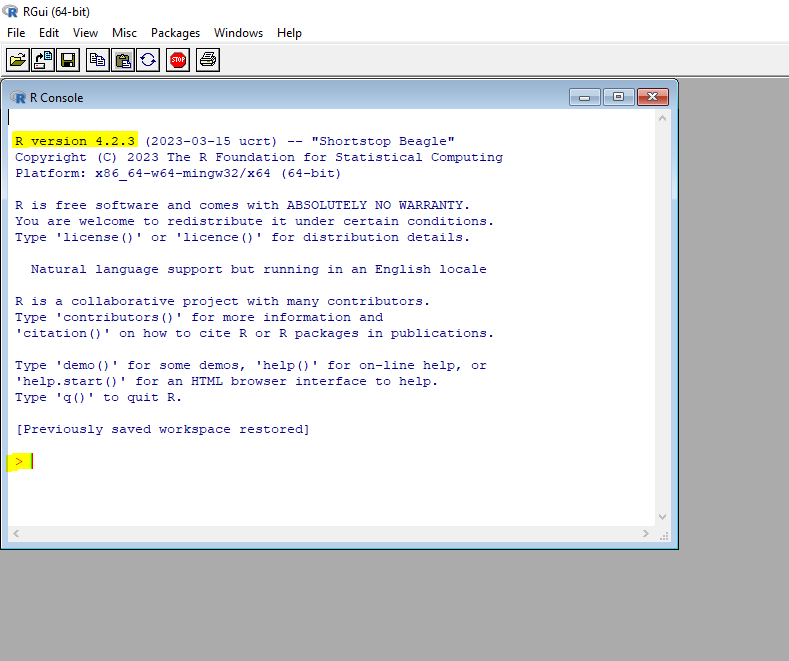
You can start using R by typing in commands after commands prompt >. To get the feel of R interface, let’s work through a simple example. We are presented with weights and ages data of 10 infants in their first year of life. We are interested in finding out distribution of the weights and their relationship with to age.
Age and Weight data are entered using a function c( ), which creates a vector of numbers or characters. The mean and standard deviation of the weights, along with the correlation between age and weight, are provided by the functions mean( ), sd( ), and cor( ), respectively. Finally, age is plotted against weight using the plot( ) function, allowing you to visually inspect the trend.
In R, variables are assigned to the values using assignment operator <-. Variables age and weight are assigned to the numeric vectors using assignment operator.
Copy and Paste the following code in the console and press ENTER:
age <- c(1,3,5,2,11,9,3,9,12,3)
weight <- c(4.4,5.3,7.2,5.2,8.5,7.3,6.0,10.4,10.2,6.1)
mean(weight)
sd(weight)
cor(age,weight)
plot(age,weight)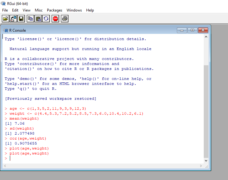
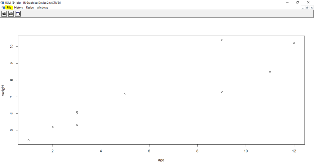
After you press the ENTER, R will plot the graph and display it in separate window. You should get two windows arranged side by side – one for the console and another for the plot.
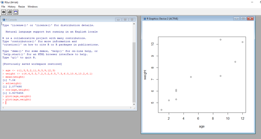
You can see from the results that the mean weight for these 10 infants is 7.06 kilograms, that the standard deviation is 2.08 kilograms, and that there is strong linear relationship between age in months and weight in kilograms (correlation = 0.91). The relationship can also be seen in the scatter plot. Not surprisingly, as infants get older, they tend to weigh more.
The [1] in front of the answer indicates a position of the output element. In our example, the output of mean(), sd() and cor() functions is single element, hence their positions are displayed as [1].
Saving R File
When you write the code running into hundreds of lines, writing all the code in the console, line by line, is not feasible.
You can use built in R editor to save your code. Go to File -> New script to open the editor, and copy paste above code into it. Name the file as “First_R_code” and save it in your folder. The R source file “First_R_code.R” with .R extension should appear into your folder. The file is also called as R script, which is list of commands in a file, written exactly as you would type them in R console.
You can open the file later for modification, save it again, and share it with another team, making the analysis work reproducible. There are some useful Script options that can be used to run the code line-by-line, print the script, and open new script. You can explore those as well.
Saving R Plots
Just as we had saved R code in a script file, we can also save R plots in various file formats including .PDF format. Open the R script again, and run it. You should get the scatter plot in separate window.
You can go to the plot window and select File -> Save as option. Select the required file format and scatter plot file will get saved into your current folder.
Summary
In this blog, we downloaded the binary R file from CRAN portal, run the executable file with default options and install R on our local machine. R is platform independent, thus runs on Windows, Mac and Linux operating systems. We explored R environment by running simple code and saving it as .R script file. We also saved the scatter plot generated from analysis.
The R interface is very basic. Professional Data Scientist often use Integrated Development Environment (IDE) to build the data analysis workflow. The integrated Development Environment has console, script, data visualization and data objects used in analysis, all displayed together in single user interface. This makes development easy, efficient and more fun. There are many IDEs available, however Rstudio is one such IDE which is widely used for reproducible data analysis in R. It is also used for literate programming.
In the next blog, we will learn more about Rstudio.